Chapter 9第9章
Using Powerful Functions: Logical, Lookup, and Database Functions使用强大的功能:逻辑、查找和数据库功能
Examples of Logical Functions逻辑函数示例
Examples of Information Functions信息功能示例
Examples of Lookup and Reference Functions查找和引用函数的示例
This chapter covers four groups of workhorse functions. 本章涵盖四组主要功能。If you process spreadsheets of medium complexity, you turn to logical and lookup functions regularly.如果您处理中等复杂度的Electron表格,则需要定期使用逻辑和查找功能。
The logical functions, including the ubiquitous逻辑函数,包括无处不在的IFfunction, help make decisions.IF函数,有助于做出决策。The information functions might be less important than they once were because Microsoft has added the信息函数可能没有以前那么重要了,因为Microsoft添加了IFERRORfunction, butINFO,CELL, andTYPEstill come in handy.IFERROR函数,但INFO、CELL和TYPE仍然很有用。The lookup functions include the powerful查找函数包括强大的VLOOKUP,MATCH, andINDIRECTfunctions.VLOOKUP、MATCH和INDIRECT函数。These functions are invaluable, particularly when you are doing something in Excel when it would be better to use Access 2019.这些功能非常宝贵,尤其是当您在Excel中执行某些操作时,使用Access 2019会更好。The database functions provide the数据库功能提供Dfunctions, such asDSUMandDMIN.D功能,如DSUM和DMIN。Even though these functions fell out of favor with the introduction of pivot tables, they are a powerful set of functions that are worthwhile to master.尽管这些函数随着pivot表的引入而不受欢迎,但它们是一组功能强大的函数,值得掌握。Linked Data Types debuted in 2018 with support for Stock Quotes and Geography.2018年推出的链接数据类型支持股票报价和地理位置。Over time, expect Excel to support more data types.随着时间的推移,Excel将支持更多的数据类型。This chapter ends with a discussion of formulas to pull data from Linked Data Types.本章最后讨论了从链接数据类型提取数据的公式。
Table 9.1 provides an alphabetical list of all the logical functions in Excel 2019. 提供Excel 2019中所有逻辑函数的字母顺序列表。Detailed examples of these functions are provided later in this chapter.本章后面将提供这些功能的详细示例。
Table 9.1 Alphabetical List of Logical Functions按字母顺序排列的逻辑函数列表
|
|
|---|---|
|
|
|
|
|
|
|
|
|
|
|
|
|
|
|
|
|
|
|
|
|
|
Table 9.2 provides an alphabetical list of the information functions in Excel 2019. 表9.2提供了Excel 2019中信息函数的字母顺序列表。Detailed examples of these functions are provided in the remainder of the chapter.本章剩余部分提供了这些功能的详细示例。
Table 9.2 Alphabetical List of Information Functions按字母顺序排列的信息功能列表
|
|
|---|---|
|
|
|
|
|
|
|
|
|
|
|
|
|
|
|
|
|
|
|
|
|
|
|
|
|
|
|
|
|
|
|
|
|
|
|
|
|
|
|
|
Table 9.3 provides an alphabetical list of the lookup functions in Excel 2019. 表9.3提供了Excel 2019中查找函数的字母顺序列表。Detailed examples of these functions are provided later in this chapter.本章后面将提供这些函数的详细示例。
Table 9.3 Alphabetical List of Lookup Functions按字母顺序排列的查找函数列表
|
|
|---|---|
|
|
|
|
|
|
|
|
|
|
|
|
|
|
|
|
|
|
|
|
|
|
|
|
|
|
|
|
|
|
|
|
|
|
|
|
|
|
|
|
|
|
|
|
|
|
|
|
|
|
|
|
Table 9.4 provides an alphabetical list of all the database functions in Excel 2019. 表9.4提供了Excel 2019中所有数据库功能的字母顺序列表。Detailed examples of these functions are provided later in this chapter.本章后面将提供这些功能的详细示例。
Table 9.4 Alphabetical List of Database Functions按字母顺序排列的数据库函数列表
|
|
|---|---|
|
|
|
|
|
|
|
|
|
|
|
|
|
|
|
|
|
|
|
|
|
|
|
|
Examples of Logical Functions逻辑函数示例
With only eight functions, the logical function group is one of the smallest in Excel. 逻辑函数组只有八个函数,是Excel中最小的函数组之一。The IF function is easy to understand, and it enables you to solve a variety of problems.IF函数很容易理解,它使您能够解决各种问题。
Using the IF Function to Make a Decision使用IF函数做出决策
IF Function to Make a DecisionMany calculations in our lives are not straightforward. 我们生活中的许多计算并不简单。Suppose that a manager offers a bonus program if her team meets its goals. 假设一位经理提供了一个奖金计划,如果她的团队达到了目标。Or perhaps a commission plan offers a bonus if a certain profit goal is met. 或者,如果达到某个利润目标,佣金计划可能会提供奖金。You can solve these types of calculations by using the 可以使用IF function.IF函数来解决这些类型的计算。
Syntax:语法:
Click here to view code image单击此处查看代码图像
IF(logical_test,value_if_true,value_if_false)
There are three arguments in the IF function. IF函数中有三个参数。The first argument is any logical test that results in a 第一个参数是任何逻辑测试,结果是TRUE or FALSE. TRUE或FALSE。For example, you might have logical tests such as these:例如,您可能有如下逻辑测试:
A2>100
B5="West"
C99<=D99
All logical tests involve one of the comparison operators shown in Table 9.5.所有逻辑测试都涉及表9.5中所示的一个比较运算符。
Table 9.5 Comparison Operators比较运算符
|
|
|
|---|---|---|
= |
|
C1=D1 |
> |
|
A1>B1 |
< |
|
A1<B1 |
>= |
|
A1>=0 |
<= |
|
A1<=99 |
<> |
|
A2<>B2 |
The remaining two arguments are the formula or value to use if the logical test is 其余两个参数是逻辑测试为TRUE and the formula or value to use if the logical test is FALSE.TRUE时使用的公式或值,以及逻辑测试为FALSE时使用的公式或值。
When you read an 阅读IF function, you should think of the first comma as the word then and the second comma as the word otherwise. IF函数时,应将第一个逗号视为单词then,将第二个逗号视作为单词otherwise。For example, 例如,=IF(A2>10,25,0) would be read as “If A2>10, then 25; otherwise, 0.”=IF(A2>10,25,0)将被解读为“如果A2>10,则为25;否则为0”
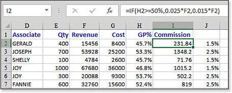
Figure 9.1 calculates a sales commission. 图9.1计算了销售佣金。The commission rate is 1.5 percent of revenue. 佣金率为收入的1.5%。However, if the gross profit percentage is 50% or higher, the commission rate is 2.5 percent of revenue.然而,如果毛利率为50%或更高,佣金率为收入的2.5%。
Note
Mathematicians would correctly note that in both the second and third arguments of the formula 数学家们会正确地注意到,在公式=IF(H2>=50%,0.025*F2,0.015*F2), you are multiplying by F2. =IF(H2>=50%,0.025*F2,0.015*F2)的第二个和第三个参数中,您是在乘以F2。Therefore, you could simplify the formula by using 因此,您可以使用=IF(H2>=50%,0.025,0.015)*F2.=IF(H2>=50%,0.025,0.015)*F2简化公式。
In this case, the logical test is 在这种情况下,逻辑测试为H2>=50%. H2>=50%。The formula for whether that test is true is 该测试是否正确的公式为0.025*F2. 0.025*F2。Otherwise, the formula is 否则,公式为0.015*F2. 0.015*F2。You could build the formula as 您可以将公式构建为:=IF(H2>=50%,0.025*F2,0.015*F2).=IF(H2>=50%,0.025*F2,0.015*F2)。
Using the AND Function to Check for Two or More Conditions使用AND函数检查两种或更多情况
AND Function to Check for Two or More ConditionsThe previous example had one simple condition: If the value in column H was greater than or equal to 50%, the commission rate changed.上一个例子有一个简单的条件:如果H列中的值大于或等于50%,佣金率就会改变。
However, in many cases, you might need to test for two or more conditions. 然而,在许多情况下,您可能需要测试两个或更多条件。For example, suppose that a retail store manager offers a $25 bonus for every leather jacket sold on Fridays this month. 例如,假设一位零售店经理为本月周五售出的每件皮夹克提供25美元的奖金。In this case, the logical test requires you to determine whether both conditions are true. 在这种情况下,逻辑测试要求您确定这两个条件是否都为真。You can do this with the 您可以使用AND function.AND函数来实现这一点。
Syntax:语法:
AND(logical1,logical2,...)
The arguments 参数logical1,logical2,... are from one to 255 expressions that evaluate to either TRUE or FALSE. logical1,logical2,...是从一到255个表达式,计算结果为TRUE或FALSE。The function returns 仅当所有参数均为TRUE only if all arguments are TRUE.TRUE时,该函数才返回TRUE。
In Figure 9.2, the function in cell F2 checks whether cell E2 is a jacket and whether the date in cell D2 falls on a Friday:在图9.2中,单元格F2中的函数检查单元格E2是否为夹套,以及单元格D2中的日期是否为周五:
=AND(E2="Jacket",WEEKDAY(D2,2)=5)
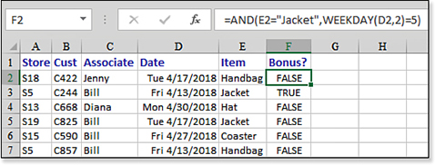
AND function is TRUE only when every condition is met.AND函数才为TRUE。Using OR to Check Whether One or More Conditions Are Met使用OR检查是否满足一个或多个条件
OR to Check Whether One or More Conditions Are MetIn the earlier examples, all the conditions had to be met for the 在前面的例子中,IF function to be true. IF函数必须满足所有条件才能为真。In other cases, you might need to identify when exactly one condition is true, or when one or more conditions are true.在其他情况下,您可能需要确定一个条件何时为真,或者一个或多个条件何时为真。
For example, a sales manager may want to reward big orders and orders from new customers. 例如,销售经理可能想要奖励大订单和新客户的订单。The manager may offer a commission bonus if the order is more than $50,000 or if the customer is a new customer this year. 如果订单金额超过50000美元,或者客户是今年的新客户,经理可以提供佣金奖金。The bonus is awarded if either condition is true. 如果其中一个条件为真,则奖励。But only one bonus is paid; you do not give two bonuses if a customer is both new and the order is large. 但只支付了一笔奖金;如果客户都是新客户,而且订单很大,你不会给两个奖金。In this case, you would use the 在这种情况下,您将使用OR function with logical tests to check whether the customer is new or if the order is large.OR函数和逻辑测试来检查客户是新客户还是订单大。
To test whether a particular sale meets either condition, use the 要测试特定销售是否满足任一条件,请使用OR function. OR函数。The 如果任一条件为OR function returns TRUE if any condition is TRUE and returns FALSE if none of the conditions are TRUE.TRUE,OR函数返回TRUE;如果没有条件均为TRUE,则返回FALSE。
Syntax:语法:
OR(logical1,logical2,...)
The OR function checks whether any of the arguments are TRUE. OR函数检查任何参数是否为TRUE。It returns a 只有当所有参数都为FALSE only if all the arguments are FALSE. FALSE时,才会返回FALSE。If any argument is 如果任何参数为TRUE, the function returns TRUE.TRUE,则函数返回TRUE。
The arguments 参数logical1,logical2,... are 1 to 255 conditions that can evaluate to TRUE or FALSE.logical1,logical2,...是1到255个条件,可以计算为TRUE或FALSE。
Nesting IF Functions Versus IFS SWITCH or CHOOSE嵌套IF函数与使用IFS SWITCH和CHOOSE的对比
IF Functions Versus IFS SWITCH or CHOOSEThe IF function offers only two possible values: Either the logical test is TRUE, and the first formula or value is used, or the logical test is FALSE and the second formula or value is used.IF函数只提供两个可能的值:逻辑测试为TRUE,使用第一个公式或值,或者逻辑测试为FALSE,使用第二个公式或数值。
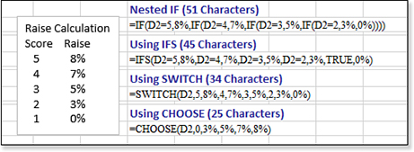
Many situations have a series of choices. For example, in a human resources department, annual merit raises might be given based on the employee’s numeric rating in an annual review in which employees are ranked on a five-point scale. 很多情况下都有一系列的选择。例如,在人力资源部门,年度绩效加薪可能基于员工在年度考核中的数字评分,员工在年度考核中按五分制进行排名。The rules for setting the raise are as follows:设定加薪的规则如下:
5: 8% raise
4: 7% raise
3: 5% raise
2: 3% raise
1: No raise
Traditionally, you would test for five conditions by nesting four IF functions:传统上,您会通过嵌套四个IF函数来测试五个条件:
Click here to view code image单击此处查看代码图像
=IF(D2=5,8%,IF(D2=4,7%,IF(D2=3,5%,IF(D2=2,3%,0%))))
You only needed four IF functions to test for five conditions. 您只需要四个IF函数就可以测试五个条件。After testing for the first four conditions, the fifth answer would be provided in the 在测试前四个条件后,第五个答案将在最后一个Value_If_False for the last IF function.IF函数的Value_If_False中提供。
In February 2017, Office 365 customers were offered two alternatives:2017年2月,Office 365客户获得了两种选择:
Click here to view code image单击此处查看代码图像
=IFS(D2=5,8%,D2=4,7%,D2=3,5%,D2=2,3%,TRUE,0%)

=SWITCH(D2,5,8%,4,7%,3,5%,2,3%,0%)
Syntax:语法:
Click here to view code image单击此处查看代码图像
IFS(logical_test1, value_if_true1, [logical_test2, value_if_true2…])
Syntax:语法:
Click here to view code image单击此处查看代码图像
SWITCH(Expression, Value1, Result1,[Default_or_value2],[Result2]…)
In the IFS function, you can handle multiple conditions without nesting new functions. 在IFS函数中,您可以在不嵌套新函数的情况下处理多个条件。The IFS means that you have multiple IF conditions. IFS表示您有多个IF条件。The IFS formula above reads, “If D2 is 5, then return 8%. 上面的IFS公式是:“如果D2为5,则返回8%。Otherwise, if D2=4, then return 7%. 否则,如果D2=4,则返回7%。Otherwise, if D2=3, then return 5%. 否则,如果D2=3,则返回5%。Otherwise, if D2=2, then return 3%.” 否则,如果D2=2,则返回3%。”The last two arguments in IFS are a little bizarre. IFS中的最后两个论点有点奇怪。You essentially want to have a value to return if none of the previous conditions are true. 如果前面的条件都不为真,您基本上希望返回一个值。You need to put a logical test that is always True. 你需要做一个始终是TRUE的逻辑测试。Explicitly typing TRUE solves the problem.显式键入TRUE可以解决这个问题。
The SWITCH function is better, in this case, because you only specify cell D2 once. 在这种情况下,切换功能更好,因为您只指定单元格D2一次。You tell the SWITCH function that you want to return a value based on the value of D2. 您告诉开关函数,您希望返回一个基于D2值的值。If it is 5, then 8%. 如果是5,则为8%。If it is 4, then 7%. 如果为4,则为7%。If it is 3, then 5%. 如果为3,则为5%。If it is 2, then 3%. 如果为2,则为3%。For any other value, use 0%. 对于任何其他值,使用0%。Note that SWITCH does not require you to enter the TRUE argument as the second-to-last argument.请注意,SWITCH不要求您输入TRUE参数作为倒数第二个参数。
In this particular case, because the five possible scores are 1 through 5, the CHOOSE function will be shortest:在这种特殊情况下,由于五个可能的分数是1到5,所以选择函数将是最短的:
=CHOOSE(D2,0,3%,5%,7%,8%)
The CHOOSE function points to a single value and then expects the value to return if the answer is 1, 2, 3, 4, 5, and so on.CHOOSE函数指向单个值,然后如果答案为1、2、3、4、5等,则期望该值返回。
Note that Excel classifies CHOOSE as a Lookup and Reference function instead of a Logical function.请注意,Excel将“选择”分类为查找和引用函数,而不是逻辑函数。

Read more about CHOOSE in “Examples of Lookup and Reference Functions” on page 244.在第244页的“查找和引用函数示例”中了解更多关于选择的信息。
Figure 9.3 compares the four formulas. 图9.3比较了四个公式。In this case, CHOOSE is the shortest.在这种情况下,CHOOSE是最短的。
Caution小心
These 这些IF formulas are hard to read. IF公式很难阅读。There is a temptation to use them for situations with very long lists of conditions. 在条件列表很长的情况下,很容易使用它们。Whereas Excel 2003 prevented you from nesting more than seven levels of Excel 2003不允许嵌套超过七个级别的IF functions, Excel 2007 and later allow you to nest up to 64 IF statements. IF函数,而Excel 2007和更高版本允许嵌套多达64个IF语句。Before you start nesting that many 在开始嵌套那么多IF statements, you should consider using VLOOKUP, which is explained later in this chapter.IF语句之前,您应该考虑使用VLOOKUP,这将在本章后面进行解释。
CHOOSE will not always be the shortest formula. CHOOSE并不总是最短的公式。SWITCH will win if you have to look for values that are not sequential or don’t have to start with 1:如果您必须查找不连续或不必以1开头的值,则SWITCH将获胜:
Click here to view code image单击此处查看代码图像
=SWITCH(A2,30,"CURRY",35,"DURANT",23,"GREEN",11,"THOMPSON","OTHER")
IFS will be better if you need to look for ranges of values:如果需要查找值的范围,IFS会更好:
Click here to view code image单击此处查看代码图像
=IFS(A2>80,"Top Tier",A2>50,"Group 2",A2>20,"Group 3",TRUE,"Bottom Tier")
Nested IF will be better if there is any chance the workbook will be opened in Excel 2016, Excel 2013, Excel 2010, or an earlier version. 如果工作簿有可能在Excel 2016、Excel 2013、Excel 2010或更早版本中打开,则嵌套IF会更好。The new IFS and SWITCH functions will return #NAME? error if opened in a prior version of Excel.新的IFS和SWITCH函数将返回#NAME?在早期版本的Excel中打开时出错。
Using the NOT Function to Simplify the Use of AND and OR
In the language of Boolean logic, there are typically NAND, NOR, and XOR functions, which stand for Not And, Not Or, and Exclusive Or. To simplify matters, Excel offers the NOT function.
Syntax:语法:
NOT(logical)
Quite simply, NOT reverses a logical value. TRUE becomes FALSE, and FALSE becomes TRUE when processed through a NOT function.
For example, suppose you need to find all flights landing outside Oklahoma. You can build a massive OR statement to find every airport code in the United States. Alternatively, you can build an OR function to find Tulsa and Oklahoma City and then use a NOT function to reverse the result: =NOT(OR(A2="Tulsa",A2="Oklahoma City")).
Using the IFERROR or IFNA Function to Simplify Error Checking
The IFERROR function, which was introduced in Excel 2007, was added at the request of many customers. To better understand the IFERROR function, you need to understand how error checking was performed during the 22 years before Excel 2007 was released.
Consider a typical spreadsheet that calculates a ratio of sales to hours. A formula of =B2/C2 returns the #DIV/0 error in the records when column C contains a zero. The typical workaround is to test for the error condition: =IF(C2=0,0,B2/C2).
In legacy versions of Excel, it was typical to use this type of IF formula on thousands of rows of data. The formula is more complex and takes longer to calculate than the new IFERROR function. However, this particular formula is tame compared to some of the formulas needed to check for errors.
A common error occurs when you use the VLOOKUP function to retrieve a value from a lookup table. In Figure 9.4, the VLOOKUP function in cell D2 asks Excel to look for the rep number S07 from cell B2 and find the corresponding name in the lookup table of F2:G9. This works great, returning JESSE from the table. However, a problem arises when the sales rep is not found in the table. In row 7, rep S09 is new and has not yet been added to the table, so Excel returns the #N/A result.

#N/A error means that the value is not in the lookup table.#N/A错误表示该值不在查找表中。If you want to avoid #N/A errors, the generally accepted workaround in legacy versions of Excel was to write this horrible formula:
Click here to view code image单击此处查看代码图像
=IF(ISNA(VLOOKUP(B7,$F$2:$G$9,2,FALSE)),"New Rep", VLOOKUP(B7,$F$2:$G$9,2,FALSE))
In English, this formula says first to find the rep name in the lookup table. If the rep is not found and returns the #N/A error, then use some other text, which in this case is the words New Rep. If the rep is found, then perform the lookup again and use that result.
Because VLOOKUP was one of the most time-intensive functions, it was horrible to have Excel perform every VLOOKUP twice in this formula. In a data set with 50,000 records, it could take minutes for the VLOOKUP to complete. Microsoft wisely added the new IFERROR function in Excel 2010 to handle all these error-checking situations.
Starting in Excel 2013, Microsoft has added the IFNA function. It works just like the IFERROR function, but the second argument is used only when the first argument results in an #N/A error. You might be able to imagine a situation in which you want to replace the #N/A errors but allow other errors to appear.
Syntax:语法:
IFERROR(value,value_if_error)
The advantage of the IFERROR function is that the calculation is evaluated only once. If the calculation results in any type of an error value, such as #N/A, #VALUE!, #REF!, #DIV/0!, #NUM!, #NAME?, or #NULL!, Excel returns the alternative value. If the calculation results in any other valid value, whether it is numeric, logical, or text, Excel returns the calculated value.
Syntax:语法:
IFNA(value,value_if_na)
If the expression evaluates to a value of #N/A, then IFNA returns value_if_na instead of the expression. Added in Excel 2013, this function replaces only #N/A errors and allows other errors to appear as the result.
The formula from the preceding section can be rewritten as =IFERROR(VLOOKUP(B7, $F$2:$G$9,2,FALSE),"New Rep") or as =IFNA(VLOOKUP(B7, $F$2:$G$9,2,FALSE),"New Rep"). Although IFNA is a bit shorter than IFERROR, the new IFNA function fails for anyone using Excel 2010 or earlier. This makes IFERROR a safer function to use for the next several years. Either IFERROR or IFNA calculates much more quickly than putting two VLOOKUPs in an IF function.
Examples of Information Functions信息功能示例
Found under the More Function icon, the 20 information functions return eclectic information about any cell. 在“更多功能”图标下,20个信息功能返回关于任何单元格的折衷信息。Eleven of the 20 functions are called the 20个函数中的11个被称为IS函数,因为它们测试各种条件。IS functions because they test for various conditions.
Using the ISFORMULA Function with Conditional Formatting to Mark Formula Cells使用带有条件格式的ISFORMULA函数标记公式单元格
ISFORMULA Function with Conditional Formatting to Mark Formula CellsThe Excel team introduced the Excel团队在Excel 2013中引入了ISFORMULA function in Excel 2013 to identify whether a cell contains a formula. ISFORMULA函数,以确定单元格是否包含公式。A hack had been floating around for years to mark formula cells using an old XL4 Macro Language function. 多年来,一个黑客一直在使用旧的XL4宏语言函数标记公式单元格。Being able to use 能够使用ISFORMULA is a great improvement.ISFORMULA是一大进步。
Syntax:语法:
ISFORMULA(reference)
Checks whether reference contains a formula. Returns TRUE or FALSE.
Figure 9.5 shows a worksheet in which all the cells have a conditional formatting formula that uses =ISFORMULA. Any cells that contain a formula are shown in white text on black fill.
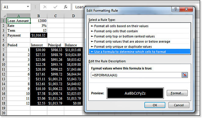
ISFORMULA function with conditional formatting to mark all the formula cells.ISFORMULA函数标记所有公式单元格。Using IS Functions to Test for Types of Values使用IS函数测试值的类型
IS Functions to Test for Types of ValuesThe remaining 剩下的IS functions enable you to test whether a cell contains numbers, text, or various other data types.IS函数允许您测试单元格是否包含数字、文本或各种其他数据类型。
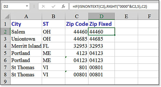
Figure 9.6 shows a common solution. Column C contains a mix of text and numeric ZIP Codes. The formula in column D, =IF(ISNONTEXT(C5),RIGHT("0000"&C5,5),C5), replaces numeric ZIP Codes with text ZIP Codes. If the value in column C is nontext, the program pads the left side of the ZIP Code with zeros and then takes the five rightmost digits.
Using the N Function to Add a Comment to a Formula使用N函数向公式添加注释
N Function to Add a Comment to a FormulaYou can call Excel’s N function a creative use for an obsolete function. Lotus 1-2-3 used to offer an N() function that converted True to 1 and False to 0. The N of any text is zero. Some have figured they could use this function to add a comment to a formula:
Click here to view code image单击此处查看代码图像
=VLOOKUP(A2,MyTable,2,False)+N("The False ensures an exact match. Don't omit False")
Using the NA Function to Force Charts to Not Plot Missing Data使用NA函数强制图表不绘制缺失数据
NA Function to Force Charts to Not Plot Missing DataSuppose that you are in charge of a school’s annual fund drive. 假设你负责一所学校的年度基金活动。Each day, you mark the fundraising total on a worksheet by following these steps:每天,您通过以下步骤在工作表上标记筹款总额:
In column A, you enter the results of each day’s collection through nine days of the fund drive (see Figure 9.7).在A列中,您输入基金驱动的九天内每天收集的结果(见图9.7)。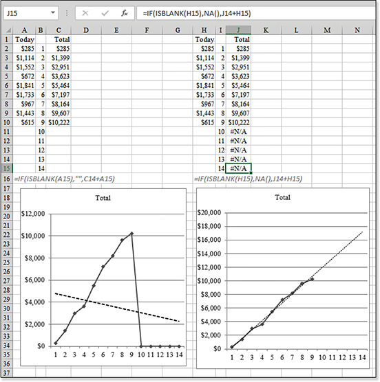
Figure 9.7 Using在右边的图表中使用NAin the chart on the right allows the trendline to ignore future missing data points and project a reasonable ending result.NA可以让趋势线忽略未来缺失的数据点,并预测合理的最终结果。You enter a formula in column C to keep track of the total collected throughout the fund drive.在C列中输入一个公式,以跟踪整个基金活动中收集的总金额。To avoid making it look like the fund drive collected nothing in days 10 through 14, you enter a formula in column C to check whether column A is blank.为了避免让它看起来像是基金驱动器在第10天到第14天没有收集到任何东西,您可以在C列中输入一个公式,以检查a列是否为空。If it is, then the如果是,则IFfunction inserts a null cell in column C. For example, the formula in cell C15 is=IF(ISBLANK(A15),"",A15+C14).IF函数在C列中插入一个空单元格。例如,单元格C15中的公式为=IF(ISBLANK(A15),"",A15+C14)。You build a line chart based on B1:C15.您将基于B1:C15构建一个折线图。You then add a trendline to the chart to predict future fundraising totals.然后在图表中添加趋势线,以预测未来的筹资总额。As shown in columns A:C of Figure 9.7, this technique fails. Even though the totals for days 10 through 14 are blank, Excel charts those days as zero. The linear trendline predicts that your fundraising will go down, with a projected total of just over $2,000.
You try the same chart again, but this time you use the
NAfunction instead of""in theIFstatement in step 3. The formula is shown in cell H16, and the results are in cell J15. Excel understands thatNAvalues should not be plotted. The trendline is calculated based on only the data points available and projects a total just under $18,000.
In many cases, you are trying to avoid #N/A! errors. However, in the case of charting a calculated column, you might want to have #N/A! produce the correct look to the chart.
Using the CELL Function to Return the Worksheet Name使用CELL函数返回工作表名称
CELL Function to Return the Worksheet NameThe CELL function can tell you information about a specific cell. Although the function can return many ancient bits of information (Excel 2003 color index, for example), it has one argument that allows you to put the worksheet name in a cell.
=CELL("filename",A1) returns the complete path, filename, and worksheet name. The technique is to locate the right square bracket at the end of the filename. Everything after that character is the worksheet tab name.
Figure 9.8 shows an example.
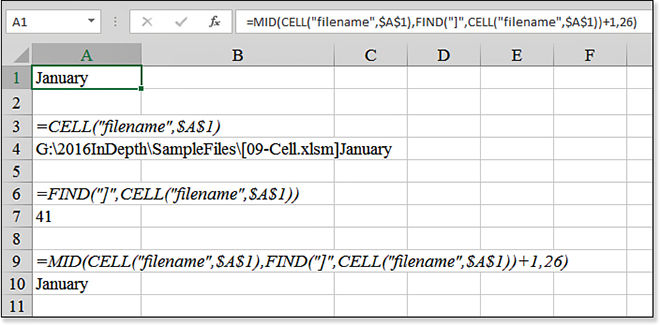
CELL function returns the full path, filename, and tab name to a cell.CELL函数返回单元格的完整路径、文件名和选项卡名。Examples of Lookup and Reference Functions查找和引用函数的示例
The Lookup & Reference icon contains 18 functions. 查找和参考图标包含18个函数。The all-star of this group is the venerable 该组的全明星是令人尊敬的VLOOKUP function, which is one of the most powerful and most used functions in Excel. VLOOKUP函数,它是Excel中功能最强大、使用最多的函数之一。As database people point out, a lot of work done in Excel should probably be done in Access. 正如数据库人员指出的那样,在Excel中完成的许多工作可能都应该在Access中完成。The VLOOKUP function enables you to perform the equivalent of a join operation in a database.VLOOKUP函数使您能够在数据库中执行相当于连接操作的操作。
This lookup and reference group also includes several functions that seem useless when considered alone. 这个查找和参考组还包括几个单独考虑时似乎无用的功能。However, when combined, they allow for some very powerful manipulations of data. 然而,当它们结合在一起时,它们允许对数据进行一些非常强大的操作。The examples in the following sections reveal details on how to use the lookup functions and how to combine them to create powerful results.以下各节中的示例详细介绍了如何使用查找函数,以及如何组合它们以创建强大的结果。
Using the CHOOSE Function for Simple Lookups使用CHOOSE函数进行简单查找
CHOOSE Function for Simple LookupsMost lookup functions require you to set up a lookup table in a range on the worksheet. 大多数查找功能要求您在工作表的某个范围内设置查找表。However, the 但是,CHOOSE function enables you to specify up to 254 choices right in the syntax of the function. CHOOSE函数允许您在函数语法中最多指定254个选项。The formula that requires the lookup should be able to calculate an integer from 1 to 254 to use the 需要查找的公式应该能够计算1到254之间的整数,以使用CHOOSE function.CHOOSE函数。
Syntax:语法:
Click here to view code image单击此处查看代码图像
CHOOSE(index_num,value1,value2,...)
The CHOOSE function chooses a value from a list of values, based on an index number. The CHOOSE function takes the following arguments:
index_num—This specifies which value argument is selected.index_nummust be a number between 1 and 254 or a formula or reference to a cell containing a number between 1 and 254:If
index_numis1,CHOOSEreturnsvalue1; if it is2,CHOOSEreturnsvalue2; and so on.If
index_numis a decimal, it is rounded down to the next lowest integer before being used.If
index_numis less than 1 or greater than the number of the last value in the list,CHOOSEreturns a#VALUE!error.
value1,value2,...—These are 1 to 254 value arguments from whichCHOOSEselects a value or an action to perform based onindex_num. The arguments can be numbers, cell references, defined names, formulas, functions, or text.
The example in Figure 9.9 shows survey data from some respondents. Columns B:F indicate their responses on five measures of your service. Column G calculates an average that ranges from 1 to 5. Suppose that you want to add words to column H to characterize the overall rating from the respondent. The following formula is used in cell H4:
Click here to view code image单击此处查看代码图像
=CHOOSE(G4,"Strongly Disagree","Disagree","Neutral","Agree","Strongly Agree")
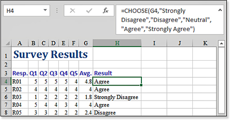
CHOOSE is great for simple choices in which the index number is between 1 and 254.CHOOSE适用于索引号介于1和254之间的简单选择。Using VLOOKUP with TRUE to Find a Value Based on a Range使用带TRUE的VLOOKUP查找基于范围的值
VLOOKUP with TRUE to Find a Value Based on a RangeVLOOKUP stands for vertical lookup. This function behaves differently, depending on the fourth parameter. This section describes using VLOOKUP in which you need to choose a value based on a table that contains ranges.
Suppose that you have a list of students and their scores on a test. 假设你有一份学生名单和他们的考试成绩。The school grading scale is based on these ranges:学校评分标准基于以下范围:
92–100 is an A.
85–91 is a B.
70–84 is a C.
65–69 is a D.
Below 65 is an F.
Follow these steps to set up a VLOOKUP for this scenario:
Because in this version of
VLOOKUPyou do not have to list every possible grade, build a table showing the scores where the grading scale changes from one grade to the next.Although the published grading scale starts with the higher values, your lookup table must be sorted in ascending sequence. This requires a bit of translation as you set up the table. Although the grading scale says that below 65 is an F, you need to set up the table to show that an F corresponds to any grade at 0 or higher. Therefore, in cell E2 enter
0, and in cell F2, enterF(see Figure 9.10).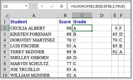
Figure 9.10 TheC列的VLOOKUPformula in column C finds the correct grade from the table in columns E and F.VLOOKUP公式从E列和F列的表格中找到正确的等级。Continue building the grading scale in successive rows of columns E and F.继续在E列和F列的连续行中构建放坡比例。Anything above a 65 is given a D.任何高于65分的成绩都被评为D。Anything above 70 is given a C.任何高于70的都会被打C。Note that this is somewhat counterintuitive because it is the opposite order that you would use if you were building a grading scale using nested请注意,这有点违反直觉,因为如果使用嵌套的IFfunctions.IF函数构建放坡比例,则会使用相反的顺序。Ensure that the numeric values are the leftmost column in your lookup table.确保数值是查找表中最左边的列。In Figure 9.10, the lookup table range is E2:F6. When you useVLOOKUP, Excel searches the first column of the lookup table for the appropriate score.When using this version of
VLOOKUPwith ranges, sort the list in ascending order. If you are not sure of the proper order, use the Sort command from the Home tab to sort the table.Because the first argument in the
VLOOKUPfunction is the student’s score, in cell C2, enter=VLOOKUP(B2,.Because the next argument is the range of the lookup table, be sure to press the F4 key after entering
E2:F6to change to an absolute reference of$E$2:$F$6.Ensure that the third argument specifies which column of the lookup table should be returned. Because the letter grade is in the second column of E2:F6, use
2for the third argument.Ensure that the final argument is either
TRUEor simply omitted. This tells Excel that you are using the sorted range variety of lookup.After you enter the formula in cell C2, again select cell C2 and double-click the fill handle to copy the formula down to all students.
Using VLOOKUP with FALSE to Find an Exact Value
In some situations, you do not want VLOOKUP to return a value based on a close match. Instead, you want Excel to find the exact match in the lookup table.
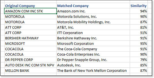
Figure 9.11 shows a table of sales. The original table had columns A through C: Rep, Date, and Sale Amount. Although a data analyst might have all the rep numbers memorized, the manager who is going to see the report prefers to have the rep names on the report.
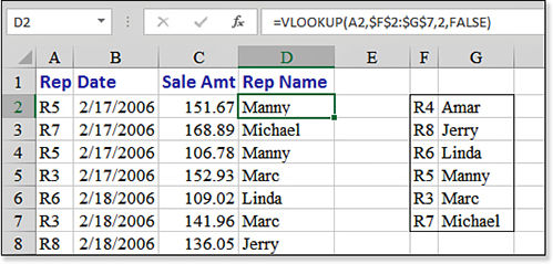
VLOOKUP needs to find the exact rep number from the table in columns E and F.VLOOKUP需要从E列和F列的表中找到确切的代表编号。To fill in the rep names from a lookup table, you follow these steps:要从查找表中填写代表姓名,请执行以下步骤:
In columns F and G, enter a table of rep numbers and rep names.在F列和G列中,输入代表编号和代表姓名表。Note that it is not important for this table to be sorted by the rep number field.请注意,此表按rep number字段排序并不重要。It is fine that the table is sorted alphabetically by name.表格按名称的字母顺序排列是可以的。Use
FALSEas the fourth parameter inVLOOKUP. You need to do this because close matches are not acceptable here. If something was sold by a new rep with number R9, you do not want to give credit to the name associated with R8 just because it is a close match.Either Excel finds an exact match and returns the result, or Excel does not give you a result.Excel会找到精确匹配并返回结果,或者Excel不会给出结果。For cell D2, you want Excel to use the rep number in A2, so in cell D2, enter
=VLOOKUP(A2,.The lookup table is in F2:G7, so enter
F2:G7and then press the F4 key to make the reference absolute. This enables you to copy the formula in step 7. After pressing F4, type a comma.In the lookup table, the rep name is in column 2 of the table, so type
2to specify that you want to return the second column of the lookup table.Finish the function with
FALSE). Press Ctrl+Enter to accept the formula and keep the cursor in cell D2.Double-click the fill handle to copy the formula down to all the rows.
VLOOKUPis a very time-intensive calculation. Having thousands ofVLOOKUPformulas significantly affects your recalculation times. In this particular case, you have successfully added rep names. It would be appropriate to convert these live formulas to their current values. Therefore, press Ctrl+C to copy. Then, from the Home tab, select Paste, Paste Values to convert the formulas to values.Note
If your lookup table is arranged sideways, with going across a row, you should use
HLOOKUP. If your data is vertical, but the key field is not the leftmost column, you can use a combination ofINDEXandMATCH, also explained later in this chapter.Look through the results.查看结果。If a sale was credited to a new rep who is not in the table, the name appears as#N/A. Manually fix these records, if needed.
To recap, the two versions of the VLOOKUP formula behave very differently. VLOOKUP with FALSE as the fourth parameter looks for an exact match, whereas VLOOKUP with TRUE as the fourth parameter looks for the closest (lower) match. In the TRUE version, the lookup table must be sorted. In the FALSE version, the table can be in any sequence. In every case, the key field must be in the left column of the lookup table.
Syntax:语法:
Click here to view code image单击此处查看代码图像
VLOOKUP(lookup_value,table_array,col_index_num,range_lookup)
VLOOKUP searches for a value in the leftmost column of a table and then returns a value in the same row from a column you specify in the table. The VLOOKUP function takes the following arguments:
lookup_value—This is the value to be found in the first column of the table.lookup_valuecan be a value, reference, or text string.table_array—This is the table of information in which data is looked up. You can use a reference to a range, such asE2:F9, or a range name such asRepTable.col_index_num—This is the column number intable_arrayfrom which the matching value must be returned. Acol_index_numvalue of1returns the value in the first column intable_array; acol_index_numvalue of2returns the value in the second column intable_array, and so on. Ifcol_index_numis less than1,VLOOKUPreturns the#VALUE!error value; ifcol_index_numis greater than the number of columns intable_array,VLOOKUPreturns the#REF!error value.range_lookup—This is a logical value that specifies whetherVLOOKUPshould find an exact match or an approximate match. If it isTRUEor omitted, an approximate match is returned. In other words, if an exact match is not found, the next largest value that is less thanlookup_valueis returned. If it isFALSE,VLOOKUPfinds an exact match. If one is not found, the error value#N/Ais returned. IfVLOOKUPcannot findlookup_valueand ifrange_lookupisTRUE, it uses the largest value that is less than or equal tolookup_value. Iflookup_valueis smaller than the smallest value in the first column oftable_array,VLOOKUPreturns an#N/Aerror. IfVLOOKUPcannot findlookup_value, andrange_lookupisFALSE,VLOOKUPreturns an#N/Aerror.
Using VLOOKUP to Match Two Lists
If Excel is used throughout your company, you undoubtedly have many lists in Excel. People use Excel to track everything. How many times are you faced with a situation in which you have two versions of a list and you need to match them up?
In Figure 9.12, the worksheet has two simple lists. Column A shows last week’s version of who was coming to an event. Column C shows this week’s version of who is coming to an event. Follow these steps if you want to find out quickly if anyone is new:
Add the heading
There?to cell D2.Because the formula in cell D3 should look at the value in cell C3 to see whether that person is in the original list in column A, start the formula with
=VLOOKUP(C3,$A$3:$A$15,.Because your only choice for the column number is to return the first column from the original list, finish the function with
1,FALSE). Then press Ctrl+Enter to accept the formula and stay in cell D3.Double-click the fill handle to copy the formula down to all rows.
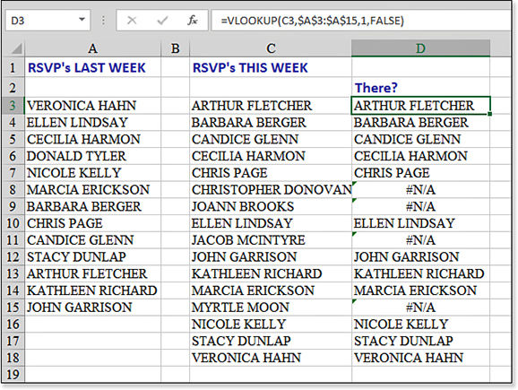
Figure 9.12 An#N/Aerror as the result ofVLOOKUPtells you that the person is new to the list.VLOOKUP的结果是一个#N/A错误,它告诉你这个人是列表中的新成员。
For any cells in which column D contains a name, it means that the person was on the RSVP list from last week. 对于D列包含姓名的任何单元格,这意味着此人从上周起就在RSVP列表中。If the result of the VLOOKUP is #N/A, you know that this person is new since the previous week.
Tip
If you study the data in Figure 9.12, you see that three more names are in the column C list than in the column A list, yet four people were reported as being new this week. This means that one of the people from last week has dropped off the list. To quickly find who dropped off the list, use the formula =VLOOKUP(A3,$C$3:$C$18,1,FALSE) in B3:B15 to find that Donald Tyler has dropped off the list.
Note that you can also use 请注意,您也可以使用MATCH to solve this problem.MATCH来解决此问题。
Using the MATCH Function to Locate the Position of a Matching Value使用MATCH函数定位匹配值的位置
MATCH Function to Locate the Position of a Matching ValueAt first glance, MATCH seems like a function that would rarely be useful. MATCH returns the relative position of an item in a range that matches a specified value in a specified order. You use MATCH instead of one of the lookup functions when you need the position of an item in a range instead of the item itself.
Suppose that your manager asks, “Can you tell me on which row I would find this value?” The manager wants to know the value or some piece of data on that record. However, rarely would the manager want to know that XYZ is found on the 111th relative row within the range A99:A11432.
MATCH comes in handy in several instances. In the first instance, consider a situation in which you are using VLOOKUP to find whether an item is in a list. In this case, you do not care what value is returned. You are interested in seeing either whether a valid value is returned, meaning that the entry is in the old list, or whether an #N/A is returned, meaning that the entry is new. In this case, using MATCH is a slightly faster way to achieve the same result.
Another handy way to use MATCH is with the INDEX function. MATCH has two features that make it more versatile than VLOOKUP. MATCH allows for wildcard matches. MATCH also allows for a search based on an exact match, based on the number just below the value, or based on a value greater than or equal to the lookup value. This third option is not available in the VLOOKUP or HLOOKUP functions.
Syntax:语法:
Click here to view code image单击此处查看代码图像
MATCH(lookup_value,lookup_array,match_type)
The MATCH function returns the relative position of an item in a column or row of values. It is useful for determining if a certain value exists in a list.
The MATCH function takes the following arguments:MATCH函数采用以下参数:
lookup_value—This is the value you use to find the value you want in a table.lookup_valuecan be a value, which is a number, text, or logical value or a cell reference to a number, text, or logical value.lookup_array—This is a contiguous range of cells that contains possible lookup values.lookup_arraycan be an array or an array reference.match_type—This is the number –1, 0, or 1. Note that you can useTRUEinstead of 1 andFALSEinstead of 0.match_typespecifies how Microsoft Excel matcheslookup_valuewith values inlookup_array. Ifmatch_typeis 1,MATCHfinds the largest value that is less than or equal tolookup_value.lookup_arraymust be placed in ascending order, such as –2, –1, 0, 1, 2,...; A–Z; orFALSE,TRUE. Ifmatch_typeis 0,MATCHfinds the first value that is exactly equal tolookup_value.lookup_arraycan be in any order. Ifmatch_typeis –1,MATCHfinds the smallest value that is greater than or equal tolookup_value.lookup_arraymust be placed in descending order, such asTRUE,FALSE; Z–A; or 2, 1, 0, –1, –2,... Ifmatch_typeis omitted, it is assumed to be 1.
MATCH returns the position of the matched value within lookup_array, not the value itself. For example, MATCH("b",{"a","b","c"},0) returns 2, the relative position of b within the array {"a","b","c"}.
MATCH does not distinguish between uppercase and lowercase letters when matching text values. If MATCH is unsuccessful in finding a match, it returns an #N/A error.
If match_type is 0 and lookup_value is text, lookup_value can contain the wildcard characters asterisk (*) and question mark (?). An asterisk matches any sequence of characters; a question mark matches any single character.
Using MATCH to Compare Two Lists
You might face situations in which you have two versions of a list, and you need to match them up.
In Figure 9.13, the worksheet has two simple lists. Column A shows last week’s list. Column C shows this week’s version of the list. You want to find out quickly which items are new. Here’s how you do it:
Add the heading
There?to cell D2.Because the formula in cell D3 looks at the value in cell C3 to see if that value is in the original list in column A, start the formula with
=MATCH(C3,$A$3:$A$11,.Because you want an exact match, use
0as the third parameter. Finish the function with a). Press Ctrl+Enter to accept the formula and stay in cell C3.Double-click the fill handle to copy the formula down to all rows.
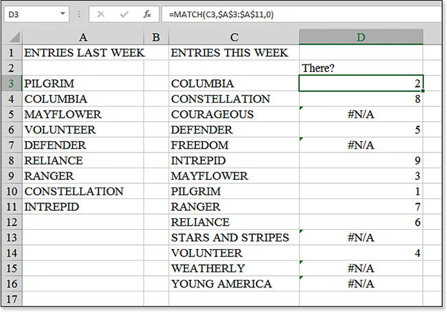
Figure 9.13 MATCHoperates slightly more quickly thanVLOOKUPand achieves the same result in this special case in which you are trying to figure out whether a value is in another list.MATCH的运行速度比VLOOKUP略快,在这个特殊情况下,您试图确定某个值是否在另一个列表中,MATCH也会获得相同的结果。
For any cells in which column D contains a number, it means that the entry was on the original list from last week. 对于D列包含数字的任何单元格,这意味着该条目位于上周的原始列表中。If the result of MATCH is #N/A, you know that this item is new since the previous week.
Using INDEX and MATCH for a Left Lookup
INDEX is another function that does not immediately seem to have many great uses. In its basic form, INDEX returns the value from a particular row and column of a rectangular range. It returns a value from a particular position of a vertical or horizontal vector.它从垂直或水平向量的特定位置返回值。
Typically, you specify a rectangular range and then indicate the row number and column number of the value that you want to return. 通常,指定一个矩形范围,然后指示要返回的值的行号和列号。In Figure 9.14, the formula in C3 returns the third row and second column of B5:D9. Certainly, this is a needlessly complicated way to point to cell C7.
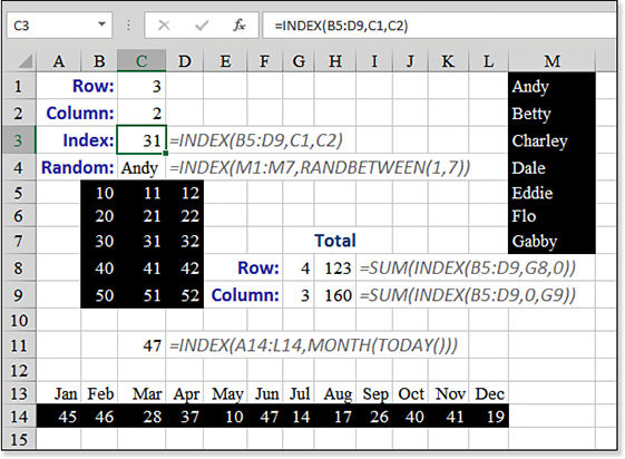
INDEX can be used in a variety of situations without the MATCH function.INDEX可以在没有MATCH函数的情况下用于各种情况。INDEX becomes interesting when you have a formula calculating the position argument. INDEX就变得有趣了。Still in Figure 9.14, a list of people is in M1:M7. You can randomly select from the list by using INDEX and RANDBETWEEN(1,7), as shown in C4.
If you specify zero as the row or column argument, INDEX returns the entire row or column. The INDEX in H8 is returning all three values from row 4 of the table, so you have to wrap the index function in a SUM or COUNT or AVERAGE function.
The data in row 14 illustrates an undocumented feature of INDEX. When the reference contains data in a single row, you can specify the column number as the second argument. To get the data for September, you can use the correct =INDEX(A14:L14,0,9) or the shortened =INDEX(A14:L14,9). In Figure 9.14, the formula in C11 returns the value from the current month by using =MONTH(TODAY()) to return a 9 as the second argument of the INDEX function. (This was written in September, hence the 9.0.)
You’ve reached Excel guru status when you start combining INDEX and MATCH. On its own, neither INDEX nor MATCH seems particularly useful. Used together, though, they become a powerful combination that is more flexible than VLOOKUP and often faster to calculate than VLOOKUP.
In Figure 9.15, a customer number is in cell B1. The customer lookup table appears in columns F, G, and H. The main problem is that the customer table does not have the customer number on the left side.主要问题是customer表的左侧没有customer编号。
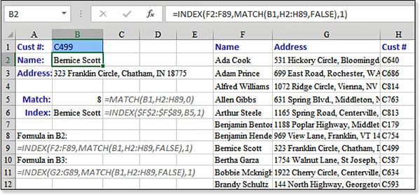
INDEX and MATCH enables you to look up data that is to the left of a key field.INDEX和MATCH的组合使您能够查找键字段左侧的数据。In many cases, you would copy column H to column E and use column E as the key of the table. However, the table in F:H is likely to be repopulated every day from a web query or an OLAP query. Therefore, it might become monotonous to move the data after every refresh. The solution is to use a combination of INDEX and MATCH. Here’s what you do:
Use the formula
=MATCH(B1,H2:H89,0)to search through column H to find the row with the customer number that matches the one in cell B1. In this case, C499 is in row 9, which is the eighth row of the table.Be sure to use exactly the same shape range as the first argument in the
INDEXfunction:=INDEX(F2:F89,WhichRow,WhichColumn)searches through the customer names in column F.For the second parameter of the
INDEXfunction, specify the relative row number. This information was provided by theMATCHfunction in step 1.Ensure that the third parameter of the
INDEXfunction is the relative column number. Because the range F2:F89 has only one column, this is either 1 or can simply be omitted.Putting the formula together, the formula in cell B2 is
=INDEX(F2:F89,MATCH(B1,H2:H89,0),1).
Syntax:语法:
Click here to view code image单击此处查看代码图像
INDEX(array,row_num,[column_num])
INDEX(reference,row_num,[column_num],[area_num])
The INDEX function returns the value at the intersection of a particular row and column within a range. This function takes the following arguments:
array—This is a range of cells or an array constant. Ifarraycontains only one row or column, the correspondingrow_numorcolumn_numargument is optional. Ifarrayhas more than one row and more than one column, and if onlyrow_numorcolumn_numis used,INDEXreturns an array of the entire row or column inarray.row_num—This selects the row inarrayfrom which to return a value. Ifrow_numis omitted,column_numis required.column_num—This selects the column inarrayfrom which to return a value. Ifcolumn_numis omitted,row_numis required.
If both the row_num and the column_num arguments are used, INDEX returns the value in the cell at the intersection of row_num and column_num.
If you set row_num or column_num to 0, INDEX returns the array of values for the entire column or row, respectively. To use values returned as an array, you use the INDEX function as an array formula in a horizontal range of cells for a row and in a vertical range of cells for a column. To enter an array formula, you press Ctrl+Shift+Enter. Thanks to modern arrays introduced in September 2018, customers using Office 365 will not need to press Ctrl+Shift+Enter.
row_num and column_num must point to a cell within array; otherwise, INDEX returns a #REF! error.
Using MATCH and INDEX to Fill a Wide Table
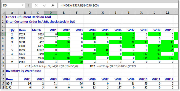
The lookup functions VLOOKUP, HLOOKUP, and MATCH can be very processor intensive when the lookup table contains hundreds of thousands of rows. The problem is worse when you have to return multiple columns from the same row of the lookup table. If it takes Excel 3 seconds to find the matching row for column 2 of the table, it will take another 3 seconds to find the matching row for column 3 of the table. If you hope to return 12 monthly columns, it could take 36 seconds.
Instead, you could find the matching row once using a MATCH function in a helper column. After the MATCH identifies the correct row, 12 INDEX functions can return the values for each month. INDEX is incredibly fast. The 13 formulas will run in 12% of the time it takes to run 12 VLOOKUP formulas.
Figure 9.16 illustrates the technique. A MATCH function in column C figures out which row contains the match. INDEX functions in D5:O12 return the monthly numbers.
MATCH functions and then 96 relatively fast INDEX functions.MATCH函数,然后执行96个相对较快的INDEX函数。Performing Many Lookups with LOOKUP使用LOOKUP执行许多查找
LOOKUPEven Excel Help tells you to avoid the old LOOKUP function. However, LOOKUP can do one useful trick that VLOOKUP and HLOOKUP cannot do—it can process many lookups in one single array formula. LOOKUP can also deal with a lookup range that is vertical and a return range that is horizontal, or vice versa.
One additional superpower of the old LOOKUP function is the capability to look up several values at once. You have to use Ctrl+Shift+Enter to accept the formula, and because LOOKUP will be returning an array of answers, you should enclose the LOOKUP in a wrapper function such as SUM to add all the results from the function.
In Figure 9.17, a series of invoices appear in rows 4 through 17. A GP% (gross profit percentage) is associated with each invoice. The sales rep will earn a bonus depending on the GP% of each invoice, as shown in E6:F10. Instead of calculating a bonus for each row, you can calculate a bonus for all the rows at once. The formula in B1 of Figure 9.17 specifies an array of B4:B17 as the lookup value. This causes Excel to perform the LOOKUP 14 times, once for each value in the range B4:B17. The formula wraps the LOOKUP results in a SUM function to add up all the bonus results. To calculate correctly, you must hold down Ctrl+Shift while pressing Enter after typing this formula. When you press Ctrl+Shift+Enter, Excel adds the curly braces around the formula. You do not type the curly braces manually. Typing the curly braces will not work.

VLOOKUP and HLOOKUP, the aging LOOKUP function can process many lookups in a single array formula.VLOOKUP和HLOOKUP不同,老迈的LOOKUP函数可以在单个数组公式中处理许多查找。As of late 2018, any Office 365 customers will have access to modern arrays. This is a major change to how Excel calculates. You will no longer have to use Ctrl+Shift+Enter in the example above. Also, with the introduction of modern arrays, every Excel function can accept an array, so you can use =SUM(VLOOKUP(B4:B17,E6:F10,2,False)), and it will calculate correctly. Modern arrays are not in Excel 2019, so those customers will still have to use 现代数组不在Excel 2019中,因此这些客户仍然必须使用LOOKUP and Ctrl+Shift+Enter.LOOKUP和Ctrl+Shift+Enter。
Using FORMULATEXT to Document a Worksheet
Quiz: Which Excel function is used the most in this book? It is FORMULATEXT. The FORMULATEXT function was added in Excel 2013. If you ask for the =FORMULATEXT(A1), Excel shows the formula that is in cell A1 as text. All the formulas shown in this book (such as cell C1 in Figure 9.17) are generated with the FORMULATEXT function.
You can use FORMULATEXT to document the formulas used in your worksheet. Normally, you can either print your worksheet with formulas showing or with the results from the formulas. By using FORMULATEXT, you can show both the formula and the result.
If you use FORMULATEXT on a cell with an array formula, the resulting text will be wrapped in curly braces that would be shown in the formula bar.
In Figure 9.18, the text of the formula shown in C3 comes from a FORMULATEXT function.
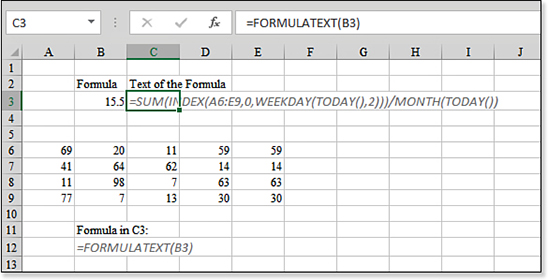
FORMULATEXT function in C3 shows the formula used in B3.FORMULATEXT函数显示了B3中使用的公式。Syntax:语法:
FORMULATEXT(reference)
This function returns a formula as text.此函数以文本形式返回公式。
Troubleshooting故障排除
FORMULATEXT fails when your reference does not contain a formula.当引用不包含公式时,FORMULATEXT失败。
There are people who had written their own versions of FormulaText as a VBA function before Excel 2013 added FormulaText. The version that was made popular on the Internet would return the formula as text if the cell contained a formula. Otherwise, it would return the value in the cell.
However, Excel’s built-in version of FORMULATEXT returns a #N/A error if the cell does not contain a formula.
One workaround is to wrap FORMULATEXT in IFNA. Instead of =FORMULATEXT(C2), use =IFNA(FORMULATEXT(C2),C2).
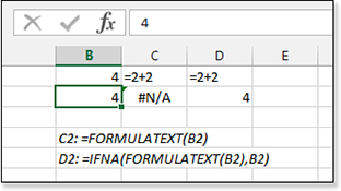
Two cells show an answer of 4. Next to each cell, a FORMULATEXT function attempts to show the formula in the adjacent cell. This works for the first cell, where the formula is =2+2. However, in the second cell, the FORMULATEXT returns a #N/A error because the cell simply contains the number 4 instead of a formula. A workaround of =IFNA(FORMULATEXT(B2),B2) will work for either formulas or values.
Using Numbers with OFFSET to Describe a Range
The language of Excel is numbers. There are functions that count the number of entries in a range. There are functions that can tell you the numeric position of a looked-up value. You might know that a particular value is found in row 20, but what if you want to perform calculations on other cells in row 20?
The OFFSET function handles this very situation. You can use OFFSET to describe a range using mostly numbers. OFFSET is flexible: It can describe a single cell, or it can describe a rectangular range.
Although INDEX can return a single cell, row, or column from a rectangular range, it has limitations. If you specify C5:Z99 as the range for an INDEX function, you can select only cells below and/or to the right of C5. The OFFSET function can move up and down or left and right from the starting cell, which is C5.
Syntax:语法:
Click here to view code image单击此处查看代码图像
OFFSET(reference,rows,cols,height,width)
The OFFSET function returns a reference to a range that is a given number of rows and columns from a given reference. This function takes the following arguments:
reference—This is the reference from which you want to base the offset.referencemust be a reference to a cell or range of adjacent cells; otherwise,OFFSETreturns a#VALUE!error.rows—This is the number of rows, up or down, that you want the upper-left cell to refer to. Using5as therowsargument, for example, specifies that the upper-left cell in the reference is five rows belowreference.rowscan be positive, which means below the starting reference, or negative, which means above the starting reference.cols—This is the number of columns to the left or right that you want the upper-left cell of the result to refer to. For example, using5as thecolsargument specifies that the upper-left cell in the reference is five columns to the right ofreference.colscan be positive, which means to the right of the starting reference, or negative, which means to the left of the starting reference. Ifrowsandcolsoffsetreferenceover the edge of the worksheet,OFFSETreturns a#REF!error. Figure 9.19 demonstrates various combinations ofrowsandcolsfrom a starting cell of cell C5.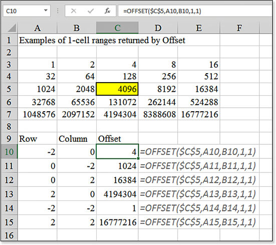
Figure 9.19 These这些OFFSETfunctions return a single cell that is a certain number of rows and columns away from cell C5.OFFSET函数返回一个单元格,该单元格与单元格C5之间有一定数量的行和列。height—This is the height, in number of rows, that you want the returned reference to be.heightmust be a positive number.width—This is the width, in number of columns, that you want the returned reference to be.widthmust be a positive number. Ifheightorwidthis omitted, Excel assumes it is the same height or width asreference.
OFFSET enables you to specify a reference. It does not move a cell. 它不会移动细胞。It does not change the selection. 它不会更改选择。It is just a numeric way to describe a reference. 这只是一种描述引用的数字方式。OFFSET can be used in any function that is expecting a reference argument.OFFSET可用于任何需要引用参数的函数。
Excel Help provides a trivial example of =SUM(OFFSET(C2,1,2,3,1)), which sums E3:E5. However, this example is silly because no one would ever write such a formula! If you were to write such a formula, you would just write =SUM(E3:E5) instead. The power of OFFSET comes when at least one of the four numeric arguments is calculated by the COUNT function or a lookup function.
In Figure 9.20, you can use COUNT(A5:A99) to count how many entries are in column A. If you assume that there are no blanks in the range of data, you can use the COUNT result as the height argument in OFFSET to describe the range of numbers. Here’s what you do:
There is nothing magical about the reference, so write it as
=OFFSET(A5,.Do not move the starting position any rows or columns from cell A5. The starting position is A5, so you always use 0 and 0 for rows and columns. Therefore, the formula is now
=OFFSET(A5,0,0,.If you want to include only the number of entries in the list, use
COUNT(A5:A999)as the height of the range. The formula is now=OFFSET(A5,0,0,COUNT(A5:A999),.The width is one column, so make the function
=OFFSET(A5,0,0,COUNT(A5:A999),1).Use your
OFFSETfunction anywhere you would normally specify a reference. You can use=SUM(OFFSET(A5,0,0,COUNT(A5:A999),1))or specify that formula as the series in a chart. This creates a dynamic chart that grows or shrinks as the number of entries changes.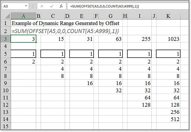
Figure 9.20 Every argument except在这些函数中,除heightis hard-coded in these functions.height外的所有参数都是硬编码的。Theheightargument comes from aCOUNTfunction to allow the range to expand as more entries are added.height参数来自一个COUNT函数,允许范围随着更多条目的添加而扩展。Troubleshooting故障排除OFFSET is a volatile function and will slow recalculation of your worksheet.偏移量是一个不稳定的函数,会减慢工作表的重新计算。Avoid OFFSET using a little-known version of INDEX.避免使用鲜为人知的索引版本进行偏移。Normally,
=INDEX(A1:A10,5)will return the value stored in the fifth row of A1:A12. Excel guru Dan Mayoh discovered an alternate use forINDEX. If theINDEXfunction is placed adjacent to a colon, theINDEXfunction returns the cell address instead of the value stored in the cell.=SUM(A1:INDEX(A1:A12,5))will sum A1:A5.Of course, you would not hard-code the 5 in the INDEX function. You might use
MONTH(TODAY())to dynamically choose the number corresponding to the current month.=SUM(A1:INDEX(A1:A12,MONTH(TODAY())))is not volatile and does the same thing as=SUM(OFFSET(A1,0,0,MONTH(TODAY()),1)).
Using INDIRECT to Build and Evaluate Cell References on the Fly
The INDIRECT function is deceivingly powerful. Consider this trivial example: In cell A1, enter the text B2. In cell B2, enter a number. In cell C3, enter the formula =INDIRECT(A1). Excel returns the number that you entered in cell B2 in cell C3. The INDIRECT function looks in cell A1 and expects to find something that is a valid cell or range reference. It then looks in that address to return the answer for the function.
The reference text can be any text that you can string together using various text functions. This enables you to create complex references that dynamically point to other sheets or to other open workbooks.
The reference text can also be a range name. You could have a validation list box in which someone selects a value from a list. If you have predefined a named range that corresponds to each possible entry on the list, INDIRECT can point to the various named ranges on the fly.
When you use traditional formulas, even absolute formulas, there is a chance that someone might insert rows or columns that will move the reference. If you need a formula to always point to cell J10, no matter how someone rearranges the worksheet, you can use =INDIRECT("J10") to handle this.
Syntax:语法:
INDIRECT(ref_text,a1)
The INDIRECT function returns the reference specified by a text string. This function takes the following arguments:
ref_text—This is a reference to a cell that contains an A1-style reference, an R1C1-style reference, a name defined as a reference, or a reference to a cell as a text string. Ifref_textis not a valid cell reference,INDIRECTreturns a#REF!error. Ifref_textrefers to an external workbook, the other workbook must be open. If the source workbook is not open,INDIRECTreturns a#REF!error.a1—This is a logical value that specifies what type of reference is contained in the cellref_text. Ifa1isTRUEor omitted,ref_textis interpreted as an A1-style reference. Ifa1isFALSE,ref_textis interpreted as an R1C1-style reference.
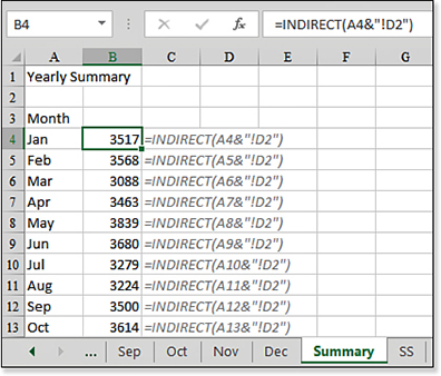
Figure 9.21 is a monthly worksheet in a workbook that has 12 similar sheets. In each worksheet, the data headings are in row 6, and the total for the worksheet appears in cell D2. To build a summary sheet that points to D2 on the individual worksheets, you can concatenate the month name from column A with “!D2” to build a reference.
Using the HYPERLINK Function to Add Hyperlinks Quickly使用HYPERLINK函数快速添加超链接
HYPERLINK Function to Add Hyperlinks QuicklyExcel enables you to add a hyperlink by using the Excel interface. Excel允许您使用Excel界面添加超链接。On the Insert tab, select the Hyperlink icon. 在“插入”选项卡上,选择超链接图标。Next, you specify text to appear in the cell and the underlying address. 接下来,指定要显示在单元格中的文本和基础地址。Building links in this way is easy, but it is tedious to build them one at a time. 以这种方式构建链接很容易,但一次构建一个链接却很乏味。If you have hundreds of links to add, you can add them quickly by using the 如果要添加数百个链接,可以使用HYPERLINK function.HYPERLINK函数快速添加。
Syntax:语法:
Click here to view code image单击此处查看代码图像
HYPERLINK(link_location,friendly_name)
The HYPERLINK function creates a shortcut that opens a document stored on your hard drive, a network server, or the Internet. This function takes the following arguments:
link_location—This is the URL address on the Internet. It could also be a path, filename, location in the same workbook, and location in another file. For example, you could link to"[C:\files\Jan2018.xls]!Sheet1!A15". Note thatlink_locationcan be a text string enclosed in quotes or a cell that contains the link.friendly_name—This is the underlined text or numeric value that is displayed in the cell.friendly_nameis displayed in blue and is underlined. Iffriendly_nameis omitted, the cell displays thelink_locationvalue as the jump text.friendly_namecan be a value, a text string, a name, or a cell that contains the jump text or value. Iffriendly_namereturns an error (for example,#VALUE!), the cell displays the error instead of the jump text.
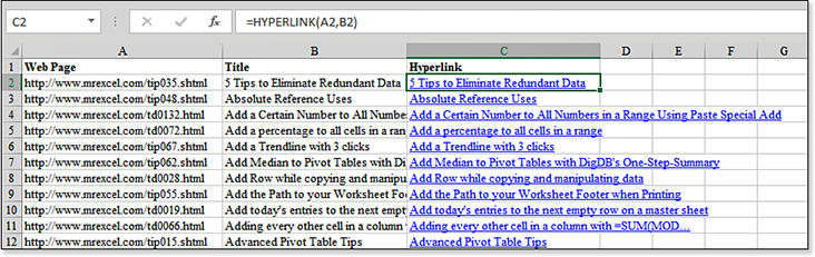
Figure 9.22 shows a list of web pages in column A. Column B contains the titles of those web pages. To quickly build a table of hyperlinks, you use =HYPERLINK(A2,B2) in cell C2 and copy the formula down the column. Unfortunately, you must keep columns A and B intact for the hyperlink to keep working. You can hide those columns, but there is no Paste Special option to convert the formula to values that will keep the hyperlink.
Note
Note that Excel does not check whether the link location is valid at the time you created the link. 请注意,Excel在创建链接时不会检查链接位置是否有效。If the link is not valid when someone clicks it, the person encounters an error.如果有人单击链接时该链接无效,则该人会遇到错误。
Tip
It is difficult to select a cell that contains a HYPERLINK function. If you click the cell, Excel attempts to follow the hyperlink. Instead, click the cell and hold the mouse button until the pointer changes from a hand to a plus. Alternatively, click a nearby cell and use the arrow keys to move to the cell with the hyperlink.
To keep only the hyperlinks, copy column C and paste to a blank Word document. Open a new workbook. Copy from Word and paste back to the new Excel document.
Alternatively, use ="#HYPERLINK("""&A2&""""&", "&""""&B2&""""&")" in C2. Copy down and paste special values. Use Find and Replace to change # to =.
Using the TRANSPOSE Function to Formulaically Turn Data
With many people using Excel in a company, there are bound to be different usage styles from person to person. Some people build their worksheets horizontally, and other people build their worksheets vertically. For example, in Figure 9.23, the monthly totals stretch horizontally across row 80. However, for some reason, you need these figures to be arranged going vertically down from cell B84.然而,由于某些原因,您需要将这些图形从单元格B84垂直向下排列。
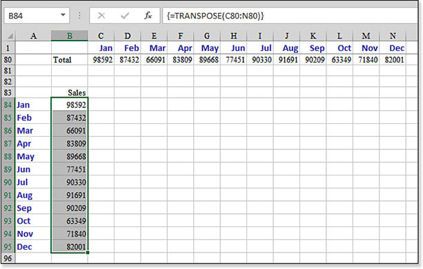
TRANSPOSE function occupies 12 cells, from B84:B95.TRANSPOSE函数占据12个单位格,来自B84:B95。The typical method is to copy C80:N80 and then use Home, Paste, Transpose. This copies a snapshot of the totals in row 80 to a column of data.
This is fine if you need only a snapshot of the totals. However, what if you want to see the totals continually updated in column B? Excel provides the TRANSPOSE function for such situations.
Because the function returns several answers, you need to use special care when entering the formula. Here’s how:
Note that C80:N80 contains 12 cells.
Select an identical number of cells starting in B84. Select B84:B95.
Even though you have 12 cells selected, type the formula,
=TRANSPOSE(C80:N80), as if you had only one cell selected.To tell Excel 2019 that this is a special type of formula called an array formula, hold down Ctrl+Shift while you press Enter. Pressing Ctrl+Shift+Enter is not required in Office 365 thanks to modern array formulas introduced in September 2018.
Excel shows the formula surrounded by curly braces in the formula bar. This is one single formula entered in 12 cells. Therefore, you cannot delete or change one cell in the range. If you want to change the formula, you need to delete all 12 cells in B84:B95 in a single command.
Syntax:语法:
TRANSPOSE(array)
The TRANSPOSE function transposes a vertical range into a horizontal array or vice versa.
The argument array is an array or a range of cells on a worksheet that you want to transpose. The transposition of an array is accomplished by using the first row of the array as the first column of the new array, the second row of the array as the second column of the new array, and so on.
Note
You can also use TRANSPOSE to turn a vertical range into a horizontal range.
Using GETPIVOTDATA to Retrieve One Cell from a Pivot Table
You might turn to this book to find out how to use most of the Excel functions. However, for the GETPIVOTDATA function, you are likely to turn to this book to find out why the function is being automatically generated for you.
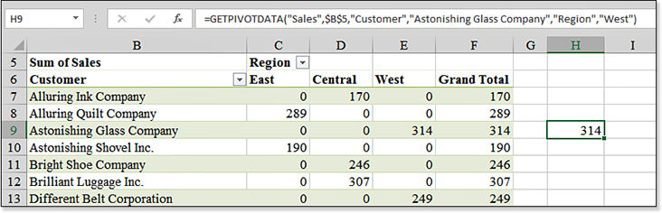
Suppose that you have a pivot table on a worksheet. You should click outside the pivot table. Next, you type an equal sign and then use the mouse to click one of the cells in the data area of the pivot table. Although you might expect this to generate a formula such as =E9, instead, Excel puts in the formula =GETPIVOTDATA("Sales",$B$5,"Customer","Astonishing Glass Company","Region","West"), as shown in Figure 9.24.
This function is annoying. As you copy the formula down to more rows, the function keeps retrieving sales to Astonishing Glass in the West region. By default, Excel is generating this function instead of a simple formula such as =E9. This happens whether you use the mouse or the arrow keys to specify the cell in the formula.
To avoid this behavior, you can enter the entire formula by manually typing it on the keyboard. Typing =E9 in a cell forces Excel to create a relative reference to cell E9. You are then free to copy the formula to other cells.
There is also a way to turn off this behavior permanently:
Select a cell inside an active pivot table.
The Pivot Table Tools tabs are displayed. Select the Analyze tab. From the PivotTable group, select the Options drop-down menu and then select the Generate GetPivotData icon. The behavior turns off.
Enter formulas by using the mouse, arrow keys, or keyboard without generating the
GETPIVOTDATAfunction.
Microsoft made GETPIVOTDATA the default behavior because the function is pretty cool. Now that you have learned how to turn off the behavior, you might want to understand exactly how it works in case you ever need to use the function.
Syntax:语法:
Click here to view code image单击此处查看代码图像
GETPIVOTDATA(data_field,pivot_table,field1,item1,field2,item2,...)
The GETPIVOTDATA function returns data stored in a pivot table report. You can use GETPIVOTDATA to retrieve summary data from a pivot table report, provided that the summary data is visible in the report. This function takes the following arguments:
data_field—This is the name, enclosed in quotation marks, for the data field that contains the data you want to retrieve.pivot_table—This is a reference to any cell, range of cells, or named range of cells in a pivot table report. This information is used to determine which pivot table report contains the data you want to retrieve.field1,item1,field2,item2,...—These are 1 to 126 pairs of field names and item names that describe the data you want to retrieve. The pairs can be in any order. Fieldnames and names for items other than dates and numbers are enclosed in quotation marks. For OLAP pivot table reports, items can contain the source name of the dimension as well as the source name of the item.
Calculated fields or items and custom calculations are included in GETPIVOTDATA calculations.
If
pivot_tableis a range that includes two or more pivot table reports, data is retrieved from whichever report was created in the range most recently.If the
fieldanditemarguments describe a single cell, the value of that cell is returned, regardless of whether it is a string, a number, an error, and so on.If an item contains a date, the value must be expressed as a serial number or populated by using the
DATEfunction so that the value is retained if the spreadsheet is opened in a different locale. For example, an item referring to the date March 5, 2015, could be entered as42068orDATE(2015,3,5). Times can be entered as decimal values or by using theTIMEfunction.If
pivot_tableis not a range in which a pivot table report is found,GETPIVOTDATAreturns#REF!. If the arguments do not describe a visible field, or if they include a page field that is not displayed,GETPIVOTDATAreturns#REF!.
Examples of Database Functions
If you were a data analyst in the 1980s and the early 1990s, you would have been enamored with the database functions. I used @DSUM every hour of my work life for many years. It was one of the most powerful weapons in any spreadsheet arsenal. Combined with a data table, the DSUM, DMIN, DMAX, and DAVERAGE functions got a serious workout when people performed data analysis in a spreadsheet.
Then, in 1993, Microsoft Excel added the pivot table to the Data menu in Excel. Pivot tables changed everything. Those powerful database functions seemed tired and worn out. Since that day in 1993, I had never used DSUM again until I created the example described in the following section. As far as I knew, the database functions had been living in a cave in South Carolina.
Maybe it is like the nostalgia of finding a box of photos of an old girlfriend, but I realized that the database functions are still pretty powerful. Customers whined enough to have Microsoft add AVERAGEIF to the COUNTIF and SUMIF arsenal. This was unnecessary: Customers could have done this easily by setting up a small criteria range and using DAVERAGE.
The database functions would be far more popular if they did not require headings for the criteria range.
The DSUM is ultra-powerful to return all records in which a specific criteria range appears (such as the region is East). However, in real life, your manager is going to want to see the records where the region is Central and West instead of East. When you start to copy the DSUM function for other regions, you realize that you need an additional two cells to hold each criteria range.
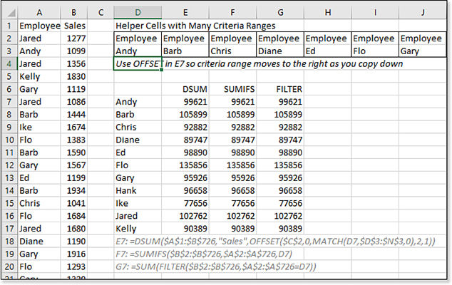
If you wanted 100 rows of DSUM to return the sales for 100 employees, you would need 200 cells of criteria range. Arranging those cells vertically would make it difficult to point to the correct criteria range. In the figure here, a blend of horizontal criteria ranges, OFFSET, and MATCH provide a method, but it will be slow to calculate. This is why you don’t see DSUM functions everywhere.
As shown in the figure, modern functions, such as SUMIFS or FILTER, provide easier ways than DSUM to arrive at the results.
Eleven of the 12 database functions are similar. DSUM, DAVERAGE, DCOUNT, DCOUNTA, DMAX, DMIN, DPRODUCT, DSTDEV, DSTDEVP, DVAR, and DVARP all perform the equivalent operation of their non-D equivalents, but they allow for complex criteria to include records that meet certain criteria. See examples of each of these in Figure 9.25.
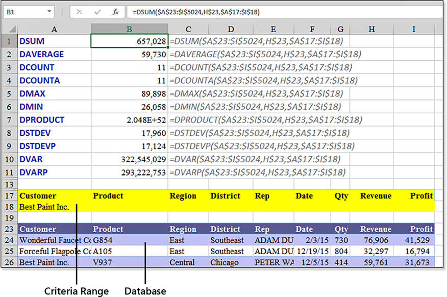
DSUM to only records for Best Paint Inc. as a customer.DSUM仅限于Best Paint Inc.作为客户的记录。To save you the hassle of looking up the confusing few, DCOUNT counts numeric cells, and DCOUNTA counts nonblank cells. DSTDEV and DVAR calculate the standard deviation and variance of a sample of a population, respectively. DSTDEVP and DVARP calculate the standard deviation and variance of the entire population, respectively. The 12th database function, DGET, has the same arguments, but it acts a bit differently, as explained later in this chapter.
Using DSUM to Conditionally Sum Records from a Database
There are three arguments to every database function. It is very easy to get your first DSUM working. The criteria argument is the one that offers vast flexibility. The following section explains the syntax for DSUM. The syntax for the other 11 database functions is identical to this.
Syntax:语法:
DSUM(database,field,criteria)
The DSUM function adds records from one field in a data set, provided that the records meet some criteria that you specify. The DSUM function takes the following arguments:
database—This is the range of cells that make up the list or database, including the heading row. Adatabaseis a list of related data in which rows of related information are records, and columns of data are fields. In Figure 9.25, the database is the 5,002 rows of data located at A23:I5024.field—This indicates which column is used in the function. You have three options when specifying a field:You can point to the cell with the
fieldname, such as H23 for Revenue.You can include the word
Revenueas thefieldargument.You can use the number
8to indicate thatRevenueis the eighth field in the database.
criteria—This is the range of cells that contains the conditions specified. You can use any range for thecriteriaargument. The criteria range typically includes at least one column label and at least one cell below the column label for specifying a condition for the column. You can also use the computed criteria discussed in “Using the Miracle Version of a Criteria Range,” later in this chapter. Learning how to create powerful criteria ranges enables you to unlock the powerful potential of the database functions. Several examples are provided in the following sections.Note
To conserve space, the remaining examples in the following sections show only the
DSUMresult. You can compare the various results to the $657,028 of revenue for the current example.
Creating a Simple Criteria Range for Database Functions
Although a criteria range needs only one field heading from the database, it is just as easy to copy the entire set of headings to a blank section of the worksheet. In Figure 9.25, for example, the headings in A17:I17, along with at least one additional row, create a criteria range.
In Figure 9.25, you see results of the 11 database functions for a simple criteria in which the customer is Best Paint Inc. Each formula specifies a database of $A$23:$I$5024. The field is H23, which is the heading for Revenue. The criteria range is A17:I18. In this example, the criteria range could have easily been A17:A18, but the A17:I18 form enables you to enter future criteria without specifying the criteria range again.
Using a Blank Criteria Range to Return All Records
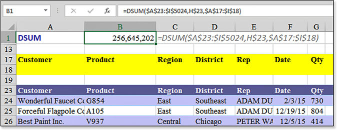
This is a trivial example, but if the second row of the criteria range is completely blank, the database function returns the total of all rows in the data set. As shown in Figure 9.26, this is $256.6 million. This is equivalent to using the SUM function.
Using AND to Join Criteria
Many people who have used SUMIF in Excel 2003 and earlier are likely to want to know how to conditionally sum based on two conditions. This is simple to do with DSUM. If two criteria are placed on the same row of the criteria range, they are joined by an AND. In Figure 9.27, for example, the $123,275 is the sum of records in which the customer is Best Paint Inc. and the product is V937.
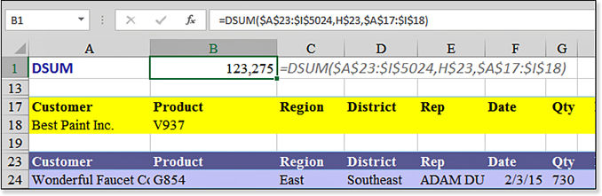
AND function; rows must meet both criteria to be included in the DSUM.AND函数连接;行必须满足这两个条件才能包含在DSUM中。Using OR to Join Criteria使用OR来连接标准
OR to Join CriteriaWhen two criteria are placed on separate rows of the criteria range, they are joined by an OR function. In Figure 9.28, the $2.1 million represents records for either Improved Radio Traders or Best Paint Inc.

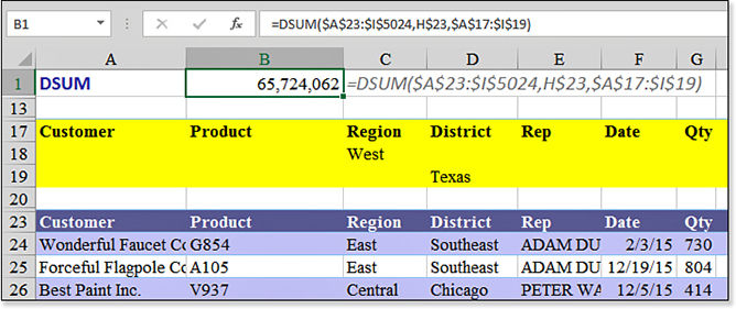
OR function; rows can meet either criterion to be included in the DSUM.You can use OR to join criteria from different fields. The criteria range in Figure 9.29 shows a Region value of West joined by an OR with a District value of Texas. This pulls a superset of all the West records plus just the Texas records, which happen to fall in the Central region.
OR can be in separate columns.Using Dates or Numbers as Criteria
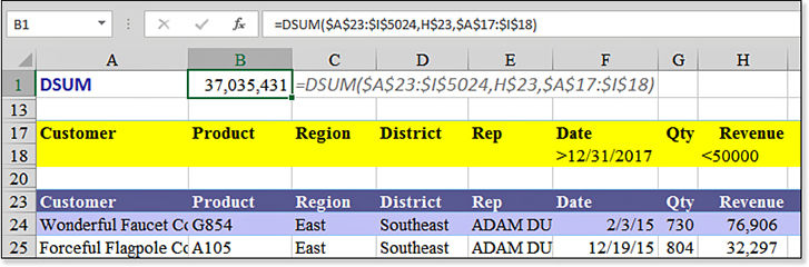
The example in Figure 9.30 finds records with a date after 2017 and with revenue under $50,000. The criteria in F18 for the date could have used any of these formats:
>12/31/2017
>=1/1/2018
>31-Dec-2017
Using the Miracle Version of a Criteria Range使用标准范围的奇迹版本
Using the criteria ranges in the preceding examples, you could easily build any complex criteria with multiple 使用前面示例中的条件范围,可以轻松地使用多个AND or OR operators.AND或OR运算符构建任何复杂的条件。
However, this could get complex. 然而,这可能会变得复杂。Imagine if you wanted to pull all the records for five specific customers and five specific products. 想象一下,如果你想获取五个特定客户和五个特定产品的所有记录。You would have to build a criteria range that is 26 rows tall. 你必须建立一个26排高的标准范围。Basically, the first row is the headings for customer and product. 基本上,第一行是客户和产品的标题。The second row indicates that you want to see records for Customer1 and Product1. 第二行表示您希望查看Customer1和Product1的记录。The third row indicates that you want to see records for Customer1 and Product2. The fourth row indicates that you want to see records for Customer1 and Product3. The seventh row indicates Customer2 and Product1. The 26th row indicates Customer5 and Product5.
If you need to pull the records for seven customers and seven products from five districts, your criteria range would grow to 246 rows tall and would probably never finish calculating.如果你需要从五个地区提取七个客户和七种产品的记录,你的标准范围将增长到246行,可能永远无法完成计算。
There is a miraculous version of the criteria range that completely avoids this problem. Here’s how it works:标准范围有一个神奇的版本,完全避免了这个问题。下面是它的工作原理:
The criteria range consists of a range that is two cells tall and one or more cells wide.标准范围包括两个单元格高和一个或多个单元格宽的范围。Contrary to instructions in Excel Help, the top cell of the criteria range cannot contain a field heading.与Excel帮助中的说明相反,条件范围的顶部单元格不能包含字段标题。The top cell must be blank or contain anything that does not match the database header row.顶部单元格必须为空或包含任何与数据库标题行不匹配的内容。For example, you could use a heading of “Computed Criteria.”例如,可以使用“计算标准”标题。The second row in the criteria range can contain any formula that evaluates to
TRUEorFALSE. This formula must point to cells in the first data row of the database. The formula can be as complex as you want provided the formula returnsTRUEorFALSE. You can combineAND,OR,VLOOKUP,NOT,MATCH, and any other functions.
For a simple example, suppose you want to find records that match one of 15 customers. You copy the customers to K24:K38. In the second row of the criteria field, write the formula =NOT(ISNA( MATCH(A24,$K$24:$K$38,0))). This formula does a MATCH on the first customer in the database to see if it is in the list in K. The ISNA and NOT functions make sure that the criteria cell returns a TRUE when the customer is one of the 15 customers.
Very quickly and without complaint, Excel compares the 5,000 rows of your database with this complex formula, and the DSUM produces the correct value, as shown in Figure 9.31.
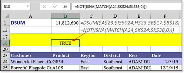
Using the DGET Function
The DGET function returns a single cell from a database. The problem is that this function is picky. If your criteria range matches zero records, DGET returns a #VALUE error. If your criteria range returns more than one row, DGET returns a #NUM! error.
To have DGET work, you need to write a criteria record that causes one and only one row to be evaluated as TRUE.
Syntax:语法:
DGET(database,field,criteria)
The DGET function returns a single cell matching criteria from a data set.DGET函数从数据集中返回单个单元格匹配条件。
Examples of Linked Data Types链接数据类型的示例
Microsoft debuted linked data types in 2018. 2018年,微软首次推出链接数据类型。The first two data types are stock market data and geographic data.前两种数据类型是股市数据和地理数据。
Enter a list of states, cities, or countries in some cells. 在某些单元格中输入州、城市或国家的列表。Select those cells and choose Geography from the Data Types gallery on the Data tab. 选择这些单元格,然后从数据选项卡上的数据类型库中选择地理位置。As shown in Figure 9.32, a Map icon appears next to each value to tell you that the cells contain a geography data type.如图9.32所示,每个值旁边都会出现一个地图图标,告诉您单元格包含地理数据类型。

If you click the map icon for a cell, a data card appears with information from Wikipedia about the state listed in the cell.如果单击某个单元格的地图图标,则会出现一张数据卡,其中包含来自维基百科的有关该单元格中所列状态的信息。
However, the more interesting feature is the new formulas that can point to the linked cell. In this example, Ohio is in H2. Go to any cell and type =H2 followed by a period. A list of fields appears. You can choose any of these fields to retrieve information about the geography. For example, =H2.Capital or =H2.Population. As shown in Figure 9.33, if the field name contains a space, wrap the name in square brackets: =H2.[Building Permits].
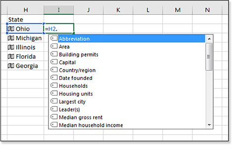
After entering the formula for the first state, you can copy the formula to pull similar data for each state. 在输入第一个状态的公式后,可以复制公式以获取每个状态的类似数据。Figure 9.34 shows the largest city in each state.图9.34显示了各州最大的城市。
![I2 shows a formula of =H2.[Largest City] and the answer is Columbus. The formula has been copied down to other states, and each row is returning the largest city from a different state.](../images/00219.jpeg)
If you type a different state name in a cell, the formulas will update. 如果在单元格中键入其他状态名称,公式将更新。In Figure 9.35, Hawaii replaced Illinois. 在图9.35中,夏威夷取代了伊利诺伊州。In a second or so, Chicago is replaced with Honolulu.在一秒钟左右的时间里,芝加哥被檀香山取代。
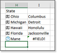
What if you mistype a name? 如果你打错名字怎么办?You will see a brand-new error value called 您将看到一个名为#FIELD!.#FIELD!的全新错误值!。
Given that this is a new feature, there are some odd limitations:鉴于这是一项新功能,有一些奇怪的限制:
The cell containing the Linked Data cannot be a formula.包含链接数据的单元格不能是公式。It must be a value. In Figure 9.35, once you have Columbus in I2, it would be nice to mark Columbus as geography and get the Columbus Ohio population with这一定是一种价值观。在图9.35中,一旦哥伦布位于I2,将哥伦布标记为地理位置并使用=I2.Population.=I2.Population获得哥伦布俄亥俄州人口将是一件好事。However, this will not work.然而,这是行不通的。My computer always includes a custom list with the U.S. states from Alabama to Wyoming.我的电脑上总是有一个从阿拉巴马州到怀俄明州的美国各州的自定义列表。This allows me to type Alabama and drag the fill handle to get the other state names.这允许我键入Alabama并拖动填充句柄来获取其他州的名称。You must be careful to drag the states before marking Alabama as a Geography type.在将阿拉巴马州列为地理类型之前,你必须小心拖拽各州。Once the cell is marked as Geography, the fill handle will not fill from custom lists.一旦单元格标记为地理位置,填充句柄将不会从自定义列表中填充。Your computer will have to be connected to the Internet to retrieve fields associated with a Linked Data Type.您的计算机必须连接到Internet才能检索与链接数据类型关联的字段。
Microsoft Labs offer a free Fuzzy Lookup add-in for Excel.微软实验室为Excel提供免费的模糊查找插件。
Doing a VLOOKUP is impossible when you have names like “ABC Corp.” and “ABC Incorporated” and “A B C”. Back in Excel 2010, the research team at Microsoft Labs created a Fuzzy Lookup add-in for Excel. The technology was cool, but Microsoft ended up adding the functionality to SQL Server instead of to Excel.
However, the add-in still works in Excel 2019 and is free from Microsoft Labs. Download from https://www.microsoft.com/en-us/download/details.aspx?id=15011.
Set the tool to return the two best matches. 将工具设置为返回两个最佳匹配项。In the figure below, there were two valid matches for Coca-Cola and a human will do a better job of knowing which one is your customer.在下图中,可口可乐有两个有效匹配项,一个人可以更好地知道哪一个是你的客户。